Introduction to Health Analytics
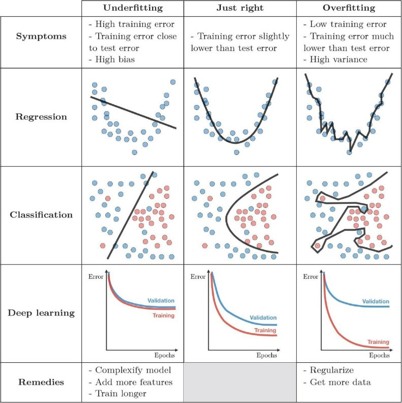
```{r setup, include=FALSE} library(tidyverse) library(gganimate) library(tidymodels) library(estimatr) library(magick) library(dagitty) library(ggthemes) library(countdown) library(marginaleffects) library(directlabels) library(ggdag) library(ggpubr) library(fixest) library(modelsummary) library(jtools) library(survival) library(survminer) library(scales) library(cowplot) library(gapminder) theme_metro <- function(x) { theme_classic() + theme(panel.background = element_rect(color = '#FAFAFA',fill='#FAFAFA'), plot.background = element_rect(color = '#FAFAFA',fill='#FAFAFA'), text = element_text(size = 16), axis.title.x = element_text(hjust = 1), axis.title.y = element_text(hjust = 1, angle = 0)) } theme_void_metro <- function(x) { theme_void() + theme(panel.background = element_rect(color = '#FAFAFA',fill='#FAFAFA'), plot.background = element_rect(color = '#FAFAFA',fill='#FAFAFA'), text = element_text(size = 16)) } theme_metro_regtitle <- function(x) { theme_classic() + theme(panel.background = element_rect(color = '#FAFAFA',fill='#FAFAFA'), plot.background = element_rect(color = '#FAFAFA',fill='#FAFAFA'), text = element_text(size = 16)) } ``` ## Today - What is machine learning - The problem of overfitting - Typology of machine learning techniques - Predicting breast cancer diagnosis with Lasso and Random Forests ## What is machine learning? ::: columns ::: {.column} {fig-align="center" fig-alt="Machine learning diagram" width=80%} ::: ::: {.column} * **AI** is the broad field of creating computer systems that perform tasks normally requiring human intelligence. These tasks include: * perception (e.g., recognizing images or speech) * reasoning and problem solving * understanding language * decision-making * **Machine learning** is a subset of AI that focuses on systems that learn patterns from data * **training**: learn from existing data * **prediction**: use what was learned to make decisions on new data ::: ::: ## Uses of AI in health analytics AI is used across the healthcare system to: - **Predict outcomes:** e.g. complications, readmissions, mortality - **Support diagnosis** e.g. image interpretation, risk scoring - **Personalise treatment** matching patients to therapies - **Improve operations**: scheduling, staffing, capacity planning ## Examples of AI tools used in healthcare | Tool | Used for | Used by | |-------------------|--------------------------------------------------------------------------|-----------------------| | Aidoc | Facilitating early disease detection and minimizing diagnostic errors | Hospitals | | Shift Technology | Streamlining claims processing and fraud detection | Insurance companies | | Atomwise | Identifying potential drug candidates and predicting their efficacy | Drug development | | BenevolentAI | Decreasing the time and expense associated with bringing new treatments to market | Drug development | | Digital Diagnostics | Detecting conditions such as diabetic retinopathy and skin cancer from medical images | Diagnostics | | PathAI | Achieving results comparable to those of experienced clinicians in diagnostics | Diagnostics | | Qventus | Enhancing operational efficiency using AI-powered predictive analytics | Healthcare facilities | | LeanTaaS | Optimizing resource allocation and reducing operational costs | Healthcare facilities | *Source: DataCamp, “AI in Healthcare”* ## What is the goal of machine learning? - Machine learning is not defined by the **type** of model used but by the **goal** - Use data to learn a rule that predicts an outcome for new observations! - At its core, machine learning is about learning a function - Given data $(X, Y)$, we want to learn a rule $f(X)$ that maps inputs $X$ to outcomes $Y$. - The goal is to choose $f(X)$ so that predictions are accurate for *new, unseen* data - Many different functions can fit the observed data! - Machine learning is about choosing between them! ## Training and testing data {fig-align="center" fig-alt="Training and testing diagram" width=70%} ## The problem of overfitting {fig-align="center" fig-alt="Machine learning diagram" width=45%} ## Machine learning methods {fig-align="center" fig-alt="Machine learning typology" width=45%} ## A basic typology of machine learning methods - Different ML methods are different ways of restricting and choosing the function $\widehat f(X)$ - **Regression + regularisation:** e.g. LASSO, ridge - Start with a standard regression model with many variables (linear, logit) - *Regularisation* shrinks or constrains coefficients in the model to prevent overfitting - **Tree-based methods:** e.g. random forests - Build the relationship using a sequence of data-driven splits in $X$ - Capture nonlinearities and interactions without specifying them in advance - Average across trees and constrain depth of trees to prevent overfitting - **Neural networks:** e.g. convolutional NNs, large language models - Construct the relationship through "layers" of nonlinear transformations - Overfitting controlled by constraining the complexity of the function - especially useful with high-dimensional or unstructured inputs (free text, images, audio) ## A note on terminology - **Feature**: a component of $X$ (or a transformation or function of it) used to predict $Y$ - **Loss**: how we measure prediction error (e.g. squared error, log loss) - **Model**: the class of functions considered - **Algorithm**: the procedure used to fit the model ## Machine learning in R: {tidymodels} ::: columns ::: {.column} * A collection of R packages for statistical modelling and machine learning. * Follows the {tidyverse} principles. * `install.packages("tidymodels")` ::: ::: {.column .center} {fig-align="center" fig-alt="tidymodels packages hex sticker logo" width=100%} Source: rpubs.com/chenx/tidymodels_tutorial ::: ::: ## Recipe and workflow ::: columns ::: {.column width="30%"} {fig-align="center" fig-alt="recipes package hex sticker" width=80%} ::: ::: {.column width="70%"} - **Recipe**: A series of preprocessing steps applied to the data *before* fitting a model, such as: - Creating dummy variables for categorical predictors - Normalizing or transforming numeric variables - Handling missing values - Creating interactions or derived features - **Workflow**: An object that bundles all steps of the modelling process, including: - Pre-processing (the `recipe`) - The model specification - Post-processing (e.g. predictions, performance metrics) - Workflows ensure the same steps are applied consistently during training, validation, and prediction. ::: ::: ## Exercise: Exploratory data analysis and standard logit - Open `health_analytics_09_ml.Rmd` for prompts. - **Load the data** Read in the `bdiag.csv` data - **Explore the data** Inspect variables, plot correlations between different variables - **Estimate a vanilla logit** Look at what goes wrong! ```{r} #| echo: false #| label: ex-1-timer countdown::countdown(minutes = 10, color_border = "#005EB8", color_text = "#005EB8", color_running_text = "white", color_running_background = "#005EB8", color_finished_text = "#005EB8", color_finished_background = "white", top = 0, margin = "1.2em", font_size = "2em") ``` # LASSO regression {background-color="#D9DBDB"} ## Linear and logistic regression models ::: columns ::: {.column} **Linear regression** ```{r} #| label: lin-reg #| eval: false #| echo: true lm(y ~ x, data = model_data) ``` {fig-align="center" fig-alt="Linear regression plot" width=70%} ::: ::: {.column .fragment} **Logistic regression** ```{r} #| label: log-reg #| eval: false #| echo: true glm(y ~ x, family = "binomial", data = model_data) ``` {fig-align="center" fig-alt="Linear regression plot" width=70%} ::: ::: # LASSO regression ## LASSO regression ::: columns ::: {.column} - **Standard regression**: chooses $\beta$ coefficients to minimize prediction error - **Least Absolute Shrinkage and Selection Operator (LASSO)**: adds a penalty for using large or many coefficients: $$ \min_{\beta} \; \text{Loss}(\beta) \;+\; \lambda \sum_j |\beta_j| $$ - Loss function depends on model choice: - **Linear regression:** sum of squared residuals (SSR) - **Logistic regression:** negative log-likelihood - **Key difference** - Regression focuses only on fit - LASSO trades off fit against model simplicity - Larger $\lambda$ pushes more coefficients towards zero - $\lambda$ is a **hyperparameter** ::: ::: {.column .fragment} {fig-align="center" fig-alt="Lambda plot for lasso regression" width=100%} Source: cvxpy.org/examples/machine_learning/lasso_regression.html ::: ::: ## Hyperparameters ::: columns ::: {.column width="40%"} - Some parts of a model are **not learned directly from the data**. - **Model parameters** (e.g. coefficients $\beta$) → estimated during training - **Hyperparameters** (e.g. $\lambda$ in LASSO) → chosen by the researcher → usually try out a variety of values and test their performance using `cross-validation' on different splits of the training data → control how the model learns - Hyperparameters affect model complexity and overfitting! ::: ::: {.column .fragment width="60%"} {fig-align="center" fig-alt="kfold validation" width=60%} Source: Introduction to Support Vector Machines and Kernel Methods. Ashfaque and Iqbal. 2019. ::: ::: # Evaluating model fit ## Evaluating model fit - In the exercise, we’ll fit **many** logistic LASSO models (different values of $\lambda$). - To choose the “best” one, we need a way to judge **predictive performance**. - Two common approaches: - **Confusion matrix** - **ROC AUC** ## Confusion matrix | | Predicted 1 | Predicted 0 | |----------------|-------------|-------------| | **Actual 1** | True Positive (TP) | False Negative (FN) | | **Actual 0** | False Positive (FP) | True Negative (TN) | - A classification model outputs **predicted probabilities**. - To create a confusion matrix, we choose a cutoff (threshold): - Predict **1** if predicted probability $\geq$ threshold - Predict **0** otherwise - A confusion matrix summarizes predictions at a **single threshold** (e.g. 0.5). - **Accuracy** $= \frac{TP + TN}{TP+TN+FP+FN}$ ## The limitation of confusion matrices - A confusion matrix depends on **choosing a threshold** to turn probabilities into classes. - Example: If $\hat p_i > 0.5$, predict “1”; otherwise “0”. - But different thresholds give different confusion matrices, and therefore different accuracy - *How do we evaluate a model without committing to one arbitrary threshold?* ## ROC curve: performance across thresholds ::: columns ::: {.column} {fig-align="center" fig-alt="ROC curve" width=100%} Source: Martin Thoma (Wikipedia) ::: ::: {.column .fragment .center} - The ROC curve varies the threshold from 0 to 1 and plots: - **True Positive Rate (TPR / sensitivity)** $$ TPR = \frac{TP}{TP+FN} $$ - **False Positive Rate (FPR)** $$ FPR = \frac{FP}{FP+TN} $$ - Each threshold $\Rightarrow$ one confusion matrix $\Rightarrow$ one point on the ROC curve. - **ROC AUC** = *area under the ROC curve* - Interpretable as: probability a randomly chosen positive case gets a higher score than a randomly chosen negative case - See [yardstick.tidymodels.org/articles/metric-types.html](https://yardstick.tidymodels.org/articles/metric-types.html). ::: ::: ## Exercise: Estimating a LASSO logistic regression in R - Split data into training and test datasets - Define training data subsets for cross-validation - Split training data into **folds** for cross-validation - Repeated cross-validation trains and validates the model many times on different subsets of the training data - Specify the model using `logistic_reg()`. - Tune the hyperparameter. - Choose the best value and fit the final model. - Evaluate the model performance. ```{r} #| echo: false #| label: ex-2-timer countdown::countdown(minutes = 10, color_border = "#005EB8", color_text = "#005EB8", color_running_text = "white", color_running_background = "#005EB8", color_finished_text = "#005EB8", color_finished_background = "white", top = 0, margin = "1.2em", font_size = "2em") ``` # Random Forests ## Decision trees ::: columns ::: {.column} A tree-like model of decisions and their possible consequences. ::: ::: {.column} {fig-align="center" fig-alt="Decision tree about walking to work and the weather" width=90%} ::: ::: ## What are Random Forests? ::: columns ::: {.column} * An ensemble method * Combines many decision trees. * Can be used for classification or regression problems. * For classification tasks, the output of the random forest is the class selected by most trees. ::: ::: {.column} {fig-align="center" fig-alt="Random Forest diagram" width=100%} Source: Tse Ki Chun (Wikimedia) ::: ::: ## Hyperparameters for random forests - **trees**: number of trees in the ensemble. - **mtry**: number of predictors that will be randomly sampled at each split when creating the tree models. - **min_n**: minimum number of data points in a node that are required for the node to be split further. ## Exercise: Random Forests in {tidymodels} - Specify a random forest model using `rand_forest()` - Tune the hyperparameters using the cross-validation folds. - Fit the final model and evaluate it. ```{r} #| echo: false #| label: ex-3-timer countdown::countdown(minutes = 10, color_border = "#005EB8", color_text = "#005EB8", color_running_text = "white", color_running_background = "#005EB8", color_finished_text = "#005EB8", color_finished_background = "white", top = 0, margin = "1.2em", font_size = "2em") ``` ## Takeaways - **Machine learning** is a subset of AI that focuses on systems that learn patterns from data - The goal is to choose a prediction rule $\hat f(X)$ that allows us to predict an outcome accurately in new data! - Models trade-off predicting accurately in the training dataset vs the risk of overfitting! ## Thank you - Please fill out the MODES survey before you leave today! - Be honest but constructive!